From excited-state calculations to TPA analysis
This workflow uses sum-over-states (SOS) theory to calculate two-photon absorption (TPA) spectra and cross sections from electronic excitation energies and dipole matrix elements. It connects Gaussian excited-state calculations and Multiwfn transition-dipole extraction with Python or MATLAB post-processing.
Theoretical basis: sum-over-states
In the electric-dipole approximation, SOS theory expresses the nonlinear optical response as sums over electronic states, using excitation energies, dipole matrix elements and frequency-dependent energy denominators. For degenerate TPA, two photons of the same frequency jointly supply the excitation energy; the intermediate-state sum describes virtual pathways, not two sequential real-state absorptions.
The post-processing code evaluates the frequency-dependent second hyperpolarizability γ, the molecular third-order optical response, with a finite set of supplied electronic states and phenomenological damping. It then uses the imaginary part of the isotropically averaged response to obtain the TPA spectrum and cross section in GM. The calculation follows the chain excitation energies and dipoles → SOS response → orientational average → TPA cross section. This is an electronic-structure-based calculation; the ML-TPA property-prediction models discussed in related publications are a separate route.
The original MATLAB repository identifies Terenziani et al. (2008) as its method reference. Orr and Ward (1971) provides the foundational perturbative SOS framework for nonlinear optical response; Göppert-Mayer (1931) is the foundational two-photon-transition paper. Full citations and DOI links are listed below.
Online calculation: upload two files
The online TPA workspace accepts one matching Gaussian .fchk + TD .log pair. After signing in with an approved account, select TPA, upload the two files and submit. The server runs the fixed Multiwfn export and Python SOS calculation; task history provides the spectrum, dipole-reference audit and a downloadable ZIP. You may close the page while it runs.
Prepare a completed all-electron, restricted closed-shell singlet TD calculation with IOp(9/40=4) and 2–40 singlet excited states. Convert the checkpoint with Gaussian formchk beforehand. Maximum sizes are 64 MiB for fchk and 16 MiB for log; the current service supports up to 300 atoms / 2000 basis functions. It checks atom order, coordinates, axes/origin, state count and energies. Incomplete, unsupported or mismatched inputs are rejected. The server does not run Gaussian or optimize a structure.
The online service accepts only the fchk + log pair. Multiwfn extraction and permanent-dipole definition checks are automatic; no text export or manually entered dipole vector is needed.
The compute portal uses a fixed HTTPS address. New access requires email verification and administrator approval. Each task uses at most 2 CPU threads / 4 GiB and has a 10-minute total limit. All tools share 1 running task, 2 queued tasks and 10 daily submissions per user. Private downloads expire after 72 hours.
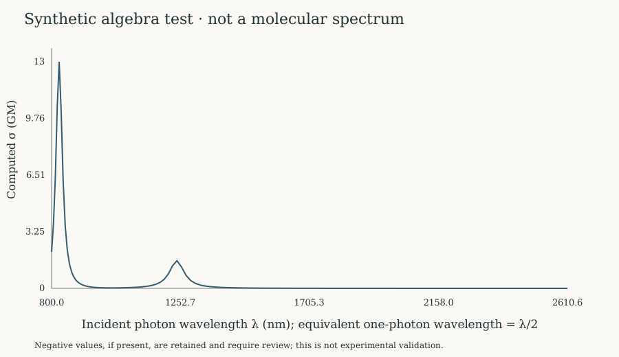
The plot above is an archived synthetic algebra verification of the numerical core, not an upload option or a molecular benchmark. Recorded verification outputs remain available for reference.
Permanent-dipole reference: save before subtracting
Every diagonal must use Δμᵢ = μᵢᵢ − μ₀₀, with a copy of μ₀₀ saved before changing any diagonal. Otherwise the first iteration zeros the reference, leaving later excited-state diagonals unchanged. The web runner uses the corrected Python implementation and checks invariance to a common shift of all permanent dipoles.
This is a definite programming error; its impact must be assessed molecule by molecule. An isolated four-molecule comparison (30 excited states per molecule), changing only this loop while keeping excitation energies, state count, damping and all other SOS expressions fixed, gave main-peak cross-section changes of +0.009%, +0.856%, +0.785% and −0.885%. Some non-main-peak samples changed by as much as 10.72% relative to their original value (within samples whose original response was at least 10% of the original peak). Small main-peak effects in these four cases cannot be generalized to other molecules, and no universal scaling factor can repair old results. Recalculate affected inputs with the corrected code; historical outputs are preserved.
In Python, save mu0 = mu[0, 0, :].copy() before the loop, then apply mu[i, i, :] -= mu0 to every diagonal. Keep .copy(): a NumPy slice without it may still change with the source matrix. Off-diagonal transition dipoles remain unchanged. Subtracted vectors must share units, coordinates and electronic/total definitions. This reference-overwrite repair and relaxed-density treatment are independent issues; the comparison does not measure a relaxed-density effect. The published correction note gives the scope and code examples.
In the pinned Multiwfn 3.8(dev), 2024-10-20 build used here, the Gaussian export has a total ground dipole and electronic excited-state diagonals. The server computes the nuclear vector from fchk nuclear charges and Cartesian coordinates, puts all permanent dipoles on a common electronic basis, and then applies the saved reference. The report and dipole_reference.csv retain raw, normalized and difference vectors. A near-zero nuclear vector is reported numerically; the electronic-only annotation alone does not demonstrate a significant mixing error in a particular historical sample.
Python companion
The existing tpa_from_multiwfn.py companion reads Multiwfn text containing the ground-state dipole, ground-to-excited and excited-to-excited transition moments, and excitation energies. Its input is the exported transition-dipole text, rather than a raw Gaussian log.
After obtaining the Python companion through the contact link above:
- Create an environment:
conda create -n tpa python=3.11, thenconda activate tpa. - Install the two dependencies:
python -m pip install numpy matplotlib. - Put the exported files in
tpa_inputsbeside the script, and runpython tpa_from_multiwfn.py --input-dir tpa_inputs --output-dir tpa_outputs --plot.
It writes tpa_summary.csv, one *_tpa_spectrum.csv per molecule, and optional PNG spectra under plots/. Python post-processing does not require MATLAB; generating new electronic-structure and dipole inputs still requires the upstream chemistry tools.
MATLAB route
The public MATLAB repository provides Gaussian and Multiwfn examples, batchTDM.bat, and calculateTPAinbatchpar.m. The public diagonal-reference loop was corrected on 2026-10-20; MATLAB execution and absolute cross sections have not been certified. It remains the public source entry for the original workflow; the Python companion is currently shared separately by enquiry.
Reading and comparing results
In the Python output, sigma_gm is the calculated cross section in GM. lambda2_nm is the incident wavelength for degenerate two-photon excitation; lambda_half_nm is half that value, the one-photon-equivalent wavelength. Keep these conventions explicit when plotting or reporting a peak.
The web runner retains the audited Python core's equations, frequency grid and constants, including its legacy 0.528 Å atomic-dipole conversion, and uses 0.05 eV denominator damping (not a certified spectral FWHM). Negative response values are retained and marked for review. The reference fix alone does not validate absolute cross sections, prefactors or state convergence. The Python and MATLAB routes implement the existing post-processing workflow. Compare a known input when switching implementations; numerical equivalence has not been certified. A finite SOS state sum requires convergence checks. Report the electronic-structure method, basis set, solvent treatment, included states, dipole inputs and damping/broadening convention when comparing cross sections; peak heights are sensitive to broadening. Match these settings between implementations.
Theory and software references
- Direct method reference named by the original workflow: F. Terenziani, C. Katan, E. Badaeva, S. Tretiak and M. Blanchard-Desce. Enhanced Two-Photon Absorption of Organic Chromophores: Theoretical and Experimental Assessments. Advanced Materials 20, 4641–4678 (2008). DOI:
10.1002/adma.200800402. - Foundational SOS response theory: B. J. Orr and J. F. Ward. Perturbation theory of the non-linear optical polarization of an isolated system. Molecular Physics 20, 513–526 (1971). DOI:
10.1080/00268977100100481. - Foundational two-photon-transition theory: M. Göppert-Mayer. Über Elementarakte mit zwei Quantensprüngen. Annalen der Physik 401 [series volume 9], 273–294 (1931). DOI:
10.1002/andp.19314010303. - Upstream wavefunction-analysis software: T. Lu and F. Chen. Multiwfn: A multifunctional wavefunction analyzer. Journal of Computational Chemistry 33, 580–592 (2012). DOI:
10.1002/jcc.22885. Cite the Multiwfn version actually used, alongside the applicable Gaussian and electronic-structure-method references.
- Current Multiwfn developments: T. Lu. A comprehensive electron wavefunction analysis toolbox for chemists, Multiwfn. Journal of Chemical Physics 161, 082503 (2024). Cite both the 2012 and 2024 Multiwfn papers in the main text, as requested by the deployed build.
Related research
This tool connects with research on machine learning of TPA, nanographenes and metal–organic layers. The repository documentation lists the related application papers. These complement the theory and upstream-software references above.